Chapter 9 Long short-term memory (LSTM) networks
In Chapter 8, we trained our first deep learning models with straightforward dense network architectures that provide a bridge for our understanding as we move from shallow learning algorithms to more complex network architectures. Those first neural network architectures are not simple compared to the kinds of models we used in Chapters 6 and 7, but it is possible to build many more different and more complex kinds of networks for prediction with text data. This chapter will focus on the family of long short-term memory networks (LSTMs) (Hochreiter and Schmidhuber 1997).
9.1 A first LSTM model
We will be using the same data from the previous chapter, described in Sections 8.1 and B.4. This data contains short text blurbs for prospective crowdfunding campaigns and whether those campaigns were successful. Our modeling goal is to predict whether a Kickstarter crowdfunding campaign was successful or not, based on the text blurb describing the campaign. Let’s start by splitting our data into training and testing sets.
library(tidyverse)

kickstarter <- read_csv("data/kickstarter.csv.gz")
kickstarter
#> # A tibble: 269,790 × 3
#> blurb state created_at
#> <chr> <dbl> <date>
#> 1 Exploring paint and its place in a digital world. 0 2015-03-17
#> 2 Mike Fassio wants a side-by-side photo of me and Hazel eati… 0 2014-07-11
#> 3 I need your help to get a nice graphics tablet and Photosho… 0 2014-07-30
#> 4 I want to create a Nature Photograph Series of photos of wi… 0 2015-05-08
#> 5 I want to bring colour to the world in my own artistic skil… 0 2015-02-01
#> 6 We start from some lovely pictures made by us and we decide… 0 2015-11-18
#> 7 Help me raise money to get a drawing tablet 0 2015-04-03
#> 8 I would like to share my art with the world and to do that … 0 2014-10-15
#> 9 Post Card don’t set out to simply decorate stories. Our goa… 0 2015-06-25
#> 10 My name is Siu Lon Liu and I am an illustrator seeking fund… 0 2014-07-19
#> # … with 269,780 more rowslibrary(tidymodels)
set.seed(1234)
kickstarter_split <- kickstarter %>%
filter(nchar(blurb) >= 15) %>%
mutate(state = as.integer(state)) %>%
initial_split()
kickstarter_train <- training(kickstarter_split)
kickstarter_test <- testing(kickstarter_split)Just as described in Chapter 8, the preprocessing needed for deep learning network architectures is somewhat different than for the models we used in Chapters 6 and 7. The first step is still to tokenize the text, as described in Chapter 2. After we tokenize, we filter to keep only how many words we’ll include in the analysis; step_tokenfilter() keeps the top tokens based on frequency in this data set.
library(textrecipes)

max_words <- 2e4
max_length <- 30

kick_rec <- recipe(~ blurb, data = kickstarter_train) %>%
  step_tokenize(blurb) %>%
  step_tokenfilter(blurb, max_tokens = max_words) %>%
  step_sequence_onehot(blurb, sequence_length = max_length)
After tokenizing, the preprocessing is different. We use step_sequence_onehot() to encode the sequences of words as integers representing each token in the vocabulary of 20,000 words, as described in detail in Section 8.2.2. This is different than the representations we used in Chapters 6 and 7, mainly because information about word sequence is encoded in this representation.
step_sequence_onehot() to preprocess text data records and encodes sequence information, unlike the document-term matrix and/or bag-of-tokens approaches we used in Chapters 7 and 6.
There are 202,092 blurbs in the training set and 67,365 in the testing set.
Like we discussed in the last chapter, we are using recipes and text-recipes for preprocessing before modeling. When we prep() a recipe, we compute or estimate statistics from the training set; the output of prep() is a recipe. When we bake() a recipe, we apply the preprocessing to a data set, either the training set that we started with or another set like the testing data or new data. The output of bake() is a data set like a tibble or a matrix.
We could have applied these prep() and bake() functions to any preprocessing recipes throughout this book, but we typically didn’t need to because our modeling workflows automated these steps.
kick_prep <- prep(kick_rec)
kick_train <- bake(kick_prep, new_data = NULL, composition = "matrix")

dim(kick_train)
#> [1] 202092 30Here we use composition = "matrix" because the Keras modeling functions operate on matrices, rather than a dataframe or tibble.
9.1.1 Building an LSTM
An LSTM is a specific kind of network architecture with feedback loops that allow information to persist through steps14 and memory cells that can learn to “remember” and “forget” information through sequences. LSTMs are well-suited for text because of this ability to process text as a long sequence of words or characters, and can model structures within text like word dependencies. LSTMs are useful in text modeling because of this memory through long sequences; they are also used for time series, machine translation, and similar problems.
Figure 9.1 depicts a high-level diagram of how the LSTM unit of a network works. In the diagram, part of the neural network, \(A\), operates on some of the input and outputs a value. During this process, some information is held inside \(A\) to make the network “remember” this updated network. Network \(A\) is then applied to the next input where it predicts new output and its memory is updated.
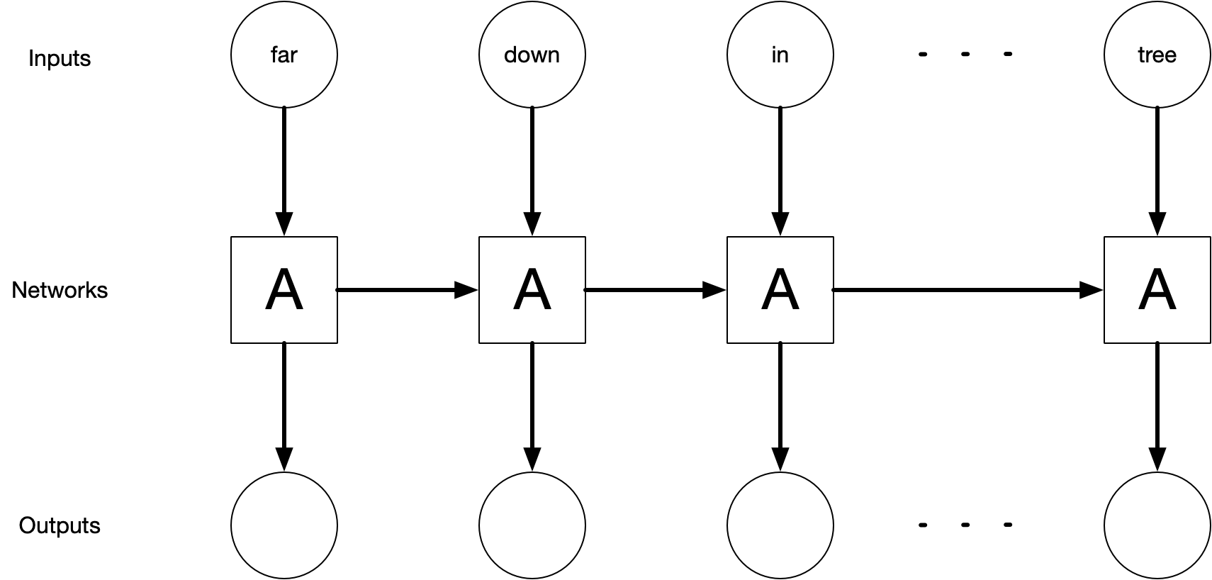
FIGURE 9.1: High-level diagram of an unrolled recurrent neural network. The recurrent neural network is the backbone of LSTM networks.
The exact shape and function of network \(A\) are beyond the reach of this book. For further study, Christopher Olah’s blog post “Understanding LSTM Networks” gives a more technical overview of how LSTM networks work.
The Keras library has convenient functions for broadly-used architectures like LSTMs so we don’t have to build it from scratch using layers; we can instead use layer_lstm(). This comes after an embedding layer that makes dense vectors from our word sequences and before a densely-connected layer for output.
library(keras)

lstm_mod <- keras_model_sequential() %>%
  layer_embedding(input_dim = max_words + 1, output_dim = 32) %>%
  layer_lstm(units = 32) %>%
  layer_dense(units = 1, activation = "sigmoid")

lstm_mod
#> Model: "sequential"
#> ________________________________________________________________________________
#> Layer (type) Output Shape Param #
#> ================================================================================
#> embedding (Embedding) (None, None, 32) 640032
#> ________________________________________________________________________________
#> lstm (LSTM) (None, 32) 8320
#> ________________________________________________________________________________
#> dense (Dense) (None, 1) 33
#> ================================================================================
#> Total params: 648,385
#> Trainable params: 648,385
#> Non-trainable params: 0
#> ________________________________________________________________________________Because we are training a binary classification model, we use activation = "sigmoid" for the last layer; we want to fit and predict to class probabilities.
Next we compile() the model, which configures the model for training with a specific optimizer and set of metrics.
"adam" (Kingma and Ba 2017), and a good loss function for binary classification is "binary_crossentropy".
lstm_mod %>%
  compile(
    optimizer = "adam",
    loss = "binary_crossentropy",
    metrics = c("accuracy")
)lstm_mod is different after we compile it, even though we didn’t assign the object to anything. This is different from how most objects in R work, so pay special attention to the state of your model objects.
After the model is compiled, we can fit it. The fit() method for Keras models has an argument validation_split that will set apart a fraction of the training data for evaluation and assessment. The performance metrics are evaluated on the validation set at the end of each epoch.
lstm_history <- lstm_mod %>%
  fit(
    kick_train,
    kickstarter_train$state,
    epochs = 10,
    validation_split = 0.25,
    batch_size = 512,
    verbose = FALSE
  )

lstm_history
#>
#> Final epoch (plot to see history):
#> loss: 0.2511
#> accuracy: 0.8816
#> val_loss: 0.7764
#> val_accuracy: 0.7571The loss on the training data (called loss here) is much better than the loss on the validation data (val_loss), indicating that we are overfitting pretty dramatically. We can see this by plotting the history as well in Figure 9.2.
plot(lstm_history)
FIGURE 9.2: Training and validation metrics for LSTM
Remember that lower loss indicates a better fitting model, and higher accuracy (closer to 1) indicates a better model.
This model continues to improve epoch after epoch on the training data, but performs worse on the validation set than the training set after the first few epochs and eventually starts to exhibit worsening performance on the validation set as epochs pass, demonstrating how extremely it is overfitting to the training data. This is very common for powerful deep learning models, including LSTMs.
9.1.2 Evaluation
We used some Keras defaults for model evaluation in the previous section, but just like we demonstrated in Section 8.2.4, we can take more control if we want or need to. Instead of using the validation_split argument, we can use the validation_data argument and send in our own validation set creating with rsample.
set.seed(234)
kick_val <- validation_split(kickstarter_train, strata = state)
kick_val
#> # Validation Set Split (0.75/0.25) using stratification
#> # A tibble: 1 × 2
#> splits id
#> <list> <chr>
#> 1 <split [151568/50524]> validationWe can access the two data sets specified by this split via the functions analysis() (the analog to training) and assessment() (the analog to testing). We need to apply our prepped preprocessing recipe kick_prep to both to transform this data to the appropriate format for our neural network architecture.
kick_analysis <- bake(kick_prep, new_data = analysis(kick_val$splits[[1]]),
                      composition = "matrix")
dim(kick_analysis)
#> [1] 151568 30kick_assess <- bake(kick_prep, new_data = assessment(kick_val$splits[[1]]),
composition = "matrix")
dim(kick_assess)#> [1] 50524 30These are each matrices appropriate for a Keras model. We will also need the outcome variables for both sets.
state_analysis <- analysis(kick_val$splits[[1]]) %>% pull(state)
state_assess <- assessment(kick_val$splits[[1]]) %>% pull(state)
Let’s also think about our LSTM model architecture. We saw evidence for significant overfitting with our first LSTM, and we can counteract that by including dropout, both in the regular sense (dropout) and in the feedback loops (recurrent_dropout).
layer_dropout().
lstm_mod <- keras_model_sequential() %>%
  layer_embedding(input_dim = max_words + 1, output_dim = 32) %>%
  layer_lstm(units = 32, dropout = 0.4, recurrent_dropout = 0.4) %>%
  layer_dense(units = 1, activation = "sigmoid")

lstm_mod %>%
  compile(
    optimizer = "adam",
    loss = "binary_crossentropy",
    metrics = c("accuracy")
  )

val_history <- lstm_mod %>%
  fit(
    kick_analysis,
    state_analysis,
    epochs = 10,
    validation_data = list(kick_assess, state_assess),
    batch_size = 512,
    verbose = FALSE
  )

val_history
#>
#> Final epoch (plot to see history):
#> loss: 0.3737
#> accuracy: 0.8271
#> val_loss: 0.6137
#> val_accuracy: 0.7357The overfitting has been reduced, and Figure 9.3 shows that the difference between our model’s performance on training and validation data is now smaller.
plot(val_history)
FIGURE 9.3: Training and validation metrics for LSTM with dropout
Remember that this is specific validation data that we have chosen ahead of time, so we can evaluate metrics flexibly in any way we need to, for example, using yardstick functions. We can create a tibble with the true and predicted values for the validation set.
val_res <- keras_predict(lstm_mod, kick_assess, state_assess)
val_res %>% metrics(state, .pred_class, .pred_1)
#> # A tibble: 4 × 3
#> .metric .estimator .estimate
#> <chr> <chr> <dbl>
#> 1 accuracy binary 0.736
#> 2 kap binary 0.470
#> 3 mn_log_loss binary 0.614
#> 4 roc_auc binary 0.805A regularized linear model trained on this data set achieved results of accuracy of 0.686 and an AUC for the ROC curve of 0.752 (Appendix C). This first LSTM with dropout is already performing better than such a linear model. We can plot the ROC curve in Figure 9.4 to evaluate the performance across the range of thresholds.
val_res %>%
  roc_curve(state, .pred_1) %>%
  autoplot()
FIGURE 9.4: ROC curve for LSTM with dropout predictions of Kickstarter campaign success
9.2 Compare to a recurrent neural network
An LSTM is actually a specific kind of recurrent neural network (RNN) (Elman 1990). Simple RNNs have feedback loops and hidden state that allow information to persist through steps but do not have memory cells like LSTMs. This difference between RNNs and LSTMs amounts to what happens in network \(A\) in Figure 9.1. RNNs tend to have a very simple structure, typically just a single tanh() layer, much simpler than what happens in LSTMs.
Simple RNNs can only connect very recent information and structure in sequences, but LSTMS can learn long-range dependencies and broader context.
Let’s train an RNN to see how it compares to the LSTM.
rnn_mod <- keras_model_sequential() %>%
  layer_embedding(input_dim = max_words + 1, output_dim = 32) %>%
  layer_simple_rnn(units = 32, dropout = 0.4, recurrent_dropout = 0.4) %>%
  layer_dense(units = 1, activation = "sigmoid")

rnn_mod %>%
  compile(
    optimizer = "adam",
    loss = "binary_crossentropy",
    metrics = c("accuracy")
  )

rnn_history <- rnn_mod %>%
  fit(
    kick_analysis,
    state_analysis,
    epochs = 10,
    validation_data = list(kick_assess, state_assess),
    batch_size = 512,
    verbose = FALSE
  )

rnn_history
#>
#> Final epoch (plot to see history):
#> loss: 0.4997
#> accuracy: 0.7651
#> val_loss: 0.5935
#> val_accuracy: 0.7136Looks like more overfitting! We can see this by plotting the history as well in Figure 9.5.
plot(rnn_history)
FIGURE 9.5: Training and validation metrics for RNN
These results are pretty disappointing overall, with worse performance than our first LSTM. Simple RNNs like the ones in this section can be challenging to train well, and just cranking up the number of embedding dimensions, units, or other network characteristics usually does not fix the problem. Often, RNNs just don’t work well compared to simpler deep learning architectures like the dense network introduced in Section 8.2 (Minaee et al. 2021), or even other machine learning approaches like regularized linear models with good preprocessing.
Fortunately, we can build on the ideas of a simple RNN with more complex architectures like LSTMs to build better-performing models.
9.3 Case study: bidirectional LSTM
The RNNs and LSTMs that we have fit so far have modeled text as sequences, specifically sequences where information and memory persists moving forward. These kinds of models can learn structures and dependencies moving forward only. In language, the structures move both directions, though; the words that come after a given structure or word can be just as important for understanding it as the ones that come before it.
We can build this into our neural network architecture with a bidirectional wrapper for RNNs or LSTMs.
A bidirectional LSTM allows the network to have both the forward and backward information about the sequences at each step.
The input sequences are passed through the network in two directions, both forward and backward, allowing the network to learn more context, structures, and dependencies.
bilstm_mod <- keras_model_sequential() %>%
  layer_embedding(input_dim = max_words + 1, output_dim = 32) %>%
  bidirectional(layer_lstm(units = 32, dropout = 0.4,
                           recurrent_dropout = 0.4)) %>%
  layer_dense(units = 1, activation = "sigmoid")

bilstm_mod %>%
  compile(
    optimizer = "adam",
    loss = "binary_crossentropy",
    metrics = c("accuracy")
  )

bilstm_history <- bilstm_mod %>%
  fit(
    kick_analysis,
    state_analysis,
    epochs = 10,
    validation_data = list(kick_assess, state_assess),
    batch_size = 512,
    verbose = FALSE
  )

bilstm_history
#>
#> Final epoch (plot to see history):
#> loss: 0.3562
#> accuracy: 0.8369
#> val_loss: 0.6246
#> val_accuracy: 0.7407The bidirectional LSTM is more able to represent the data well, but with the same amount of dropout, we do see more dramatic overfitting. Still, there is some improvement on the validation set as well.
bilstm_res <- keras_predict(bilstm_mod, kick_assess, state_assess)
bilstm_res %>% metrics(state, .pred_class, .pred_1)
#> # A tibble: 4 × 3
#> .metric .estimator .estimate
#> <chr> <chr> <dbl>
#> 1 accuracy binary 0.741
#> 2 kap binary 0.480
#> 3 mn_log_loss binary 0.625
#> 4 roc_auc binary 0.807This bidirectional LSTM, able to learn both forward and backward text structures, provides some improvement over the regular LSTM on the validation set (which had an accuracy of 0.736).
9.4 Case study: stacking LSTM layers
Deep learning architectures can be built up to create extremely complex networks. For example, RNN and/or LSTM layers can be stacked on top of each other, or together with other kinds of layers. The idea of this stacking is to increase the ability of a network to represent the data well.
Intermediate layers must be set up to return sequences (with return_sequences = TRUE) instead of the last output for each sequence.
Let’s start by adding one single additional layer.
stacked_mod <- keras_model_sequential() %>%
  layer_embedding(input_dim = max_words + 1, output_dim = 32) %>%
  layer_lstm(units = 32, dropout = 0.4, recurrent_dropout = 0.4,
             return_sequences = TRUE) %>%
  layer_lstm(units = 32, dropout = 0.4, recurrent_dropout = 0.4) %>%
  layer_dense(units = 1, activation = "sigmoid")

stacked_mod %>%
  compile(
    optimizer = "adam",
    loss = "binary_crossentropy",
    metrics = c("accuracy")
  )

stacked_history <- stacked_mod %>%
  fit(
    kick_analysis,
    state_analysis,
    epochs = 10,
    validation_data = list(kick_assess, state_assess),
    batch_size = 512,
    verbose = FALSE
  )

stacked_history
#>
#> Final epoch (plot to see history):
#> loss: 0.3714
#> accuracy: 0.8291
#> val_loss: 0.607
#> val_accuracy: 0.7361Adding another separate layer in the forward direction appears to have improved the network, about as much as extending the LSTM layer to handle information in the backward direction via the bidirectional LSTM.
stacked_res <- keras_predict(stacked_mod, kick_assess, state_assess)
stacked_res %>% metrics(state, .pred_class, .pred_1)
#> # A tibble: 4 × 3
#> .metric .estimator .estimate
#> <chr> <chr> <dbl>
#> 1 accuracy binary 0.736
#> 2 kap binary 0.471
#> 3 mn_log_loss binary 0.607
#> 4 roc_auc binary 0.806We can gradually improve a model by changing and adding to its architecture.
9.5 Case study: padding
One of the most important themes of this book is that text must be heavily preprocessed in order to be useful for machine learning algorithms, and these preprocessing decisions have big effects on model results. One decision that seems like it may not be all that important is how sequences are padded for a deep learning model. The matrix that is used as input for a neural network must be rectangular, but the training data documents are typically all different lengths. Sometimes, like in the case of the Supreme Court opinions, the lengths vary a lot; sometimes, like with the Kickstarter data, the lengths vary a little bit.
Either way, the sequences that are too long must be truncated and the sequences that are too short must be padded, typically with zeroes. This does literally mean that words or tokens are thrown away for the long documents and zeroes are added to the shorter documents, with the goal of creating a rectangular matrix that can be used for computation.
It is possible to set up an LSTM network that works with sequences of varied length; this can sometimes improve performance but takes more work to set up and is outside the scope of this book.
The default in textrecipes, as well as most deep learning for text, is padding = "pre", where zeroes are added at the beginning, and truncating = "pre", where values at the beginning are removed. What happens if we change one of these defaults?
padding_rec <- recipe(~ blurb, data = kickstarter_train) %>%
  step_tokenize(blurb) %>%
  step_tokenfilter(blurb, max_tokens = max_words) %>%
  step_sequence_onehot(blurb, sequence_length = max_length, padding = "post")

padding_prep <- prep(padding_rec)
padding_matrix <- bake(padding_prep, new_data = NULL, composition = "matrix")
dim(padding_matrix)
#> [1] 202092 30This matrix has the same dimensions as kick_train but instead of padding with zeroes at the beginning of these Kickstarter blurbs, this matrix is padded with zeroes at the end. (This preprocessing strategy still truncates longer sequences in the same way.)
pad_analysis <- bake(padding_prep, new_data = analysis(kick_val$splits[[1]]),
                     composition = "matrix")
pad_assess <- bake(padding_prep, new_data = assessment(kick_val$splits[[1]]),
                   composition = "matrix")
Now, let’s create and fit an LSTM to this preprocessed data.
padding_mod <- keras_model_sequential() %>%
  layer_embedding(input_dim = max_words + 1, output_dim = 32) %>%
  layer_lstm(units = 32, dropout = 0.4, recurrent_dropout = 0.4) %>%
  layer_dense(units = 1, activation = "sigmoid")

padding_mod %>%
  compile(
    optimizer = "adam",
    loss = "binary_crossentropy",
    metrics = c("accuracy")
  )

padding_history <- padding_mod %>%
  fit(
    pad_analysis,
    state_analysis,
    epochs = 10,
    validation_data = list(pad_assess, state_assess),
    batch_size = 512,
    verbose = FALSE
  )

padding_history
#>
#> Final epoch (plot to see history):
#> loss: 0.417
#> accuracy: 0.8031
#> val_loss: 0.598
#> val_accuracy: 0.7238This padding strategy results in noticeably worse performance than the default option!
padding_res <- keras_predict(padding_mod, pad_assess, state_assess)
padding_res %>% metrics(state, .pred_class, .pred_1)
#> # A tibble: 4 × 3
#> .metric .estimator .estimate
#> <chr> <chr> <dbl>
#> 1 accuracy binary 0.724
#> 2 kap binary 0.447
#> 3 mn_log_loss binary 0.598
#> 4 roc_auc binary 0.793The same model architecture with default padding preprocessing resulted in an accuracy of 0.736 and an AUC of 0.805; changing to padding = "post" has resulted in a remarkable degrading of predictive capacity. This result is typically attributed to the RNN/LSTM’s hidden states being flushed out by the added zeroes, before getting to the text itself.
Different preprocessing strategies have a huge impact on deep learning results.
9.6 Case study: training a regression model
All our deep learning models for text so far have used the Kickstarter crowdfunding blurbs to predict whether the campaigns were successful or not, a classification problem. In our experience, classification is more common than regression tasks with text data, but these techniques can be used for either kind of supervised machine learning question. Let’s return to the regression problem of Chapter 6 and predict the year of United States Supreme Court decisions, starting out by splitting into training and testing sets.
library(scotus)
set.seed(1234)
scotus_split <- scotus_filtered %>%
  mutate(
    year = (as.numeric(year) - 1920) / 50,
    text = str_remove_all(text, "'")
  ) %>%
  initial_split(strata = year)

scotus_train <- training(scotus_split)
scotus_test <- testing(scotus_split)
Notice that we also shifted (subtracted) and scaled (divided) the year outcome by constant factors so all the values are centered around zero and not too large. Neural networks for regression problems typically behave better when dealing with outcomes that are roughly between −1 and 1.
Next, let’s build a preprocessing recipe for these Supreme Court decisions. These documents are much longer than the Kickstarter blurbs, many thousands of words long instead of just a handful. Let’s try keeping the size of our vocabulary the same (max_words) but we will need to increase the sequence length information we store (max_length) by a great deal.
max_words <- 2e4
max_length <- 1e3

scotus_rec <- recipe(~ text, data = scotus_train) %>%
  step_tokenize(text) %>%
  step_tokenfilter(text, max_tokens = max_words) %>%
  step_sequence_onehot(text, sequence_length = max_length)

scotus_prep <- prep(scotus_rec)
scotus_train_baked <- bake(scotus_prep,
                           new_data = scotus_train,
                           composition = "matrix")
scotus_test_baked <- bake(scotus_prep,
                          new_data = scotus_test,
                          composition = "matrix")
What does our training data look like now?
dim(scotus_train_baked)#> [1] 7498 1000We only have 7498 rows of training data, and because these documents are so long and we want to keep more of each sequence, the training data has 1000 columns. You are probably starting to guess that we are going to run into problems.
Let’s create an LSTM and see what we can do. We will need to use higher-dimensional embeddings, since our sequences are much longer (we may want to increase the number of units as well, but will leave that out for the time being). Because we are training a regression model, there is no activation function for the last layer; we want to fit and predict to arbitrary values for the year.
A good default loss function for regression is mean squared error, “mse”.
scotus_mod <- keras_model_sequential() %>%
  layer_embedding(input_dim = max_words + 1, output_dim = 64) %>%
  layer_lstm(units = 32, dropout = 0.4, recurrent_dropout = 0.4) %>%
  layer_dense(units = 1)

scotus_mod %>%
  compile(
    optimizer = "adam",
    loss = "mse",
    metrics = c("mean_squared_error")
  )

scotus_history <- scotus_mod %>%
  fit(
    scotus_train_baked,
    scotus_train$year,
    epochs = 10,
    validation_split = 0.25,
    verbose = FALSE
  )
How does this model perform on the test data? Let’s transform back to real values for year so our metrics will be on the same scale as in Chapter 6.
scotus_res <- tibble(year = scotus_test$year,
                     .pred = predict(scotus_mod, scotus_test_baked)[, 1]) %>%
  mutate(across(everything(), ~ . * 50 + 1920))

scotus_res %>% metrics(year, .pred)
#> # A tibble: 3 × 3
#> .metric .estimator .estimate
#> <chr> <chr> <dbl>
#> 1 rmse standard 25.8
#> 2 rsq standard 0.777
#> 3 mae standard 18.8This is much worse than the final regularized linear model trained in Section 6.9, with an RMSE almost a decade worth of years worse. It’s possible we may be able to do a little better than this simple LSTM, but as this chapter has demonstrated, our improvements will likely not be enormous compared to the first LSTM baseline.
The main problem with this regression model is that there isn’t that much data to start with; this is an example where a deep learning model is not a good choice and we should stick with a different machine learning algorithm like regularized regression.
9.7 Case study: vocabulary size
In this chapter so far, we’ve worked with a vocabulary of 20,000 words or tokens. This is a hyperparameter of the model, and could be tuned, as we show in detail in Section 10.6. Instead of tuning in this chapter, let’s try a smaller value, corresponding to faster preprocessing and model fitting but a less powerful model, and explore whether and how much it affects model performance.
max_words <- 1e4
max_length <- 30

smaller_rec <- recipe(~ blurb, data = kickstarter_train) %>%
  step_tokenize(blurb) %>%
  step_tokenfilter(blurb, max_tokens = max_words) %>%
  step_sequence_onehot(blurb, sequence_length = max_length)

kick_prep <- prep(smaller_rec)
kick_analysis <- bake(kick_prep, new_data = analysis(kick_val$splits[[1]]),
                      composition = "matrix")
kick_assess <- bake(kick_prep, new_data = assessment(kick_val$splits[[1]]),
                    composition = "matrix")
Once our preprocessing is done and applied to our validation split kick_val, we can set up our model, another straightforward LSTM neural network.
smaller_mod <- keras_model_sequential() %>%
  layer_embedding(input_dim = max_words + 1, output_dim = 32) %>%
  layer_lstm(units = 32, dropout = 0.4, recurrent_dropout = 0.4) %>%
  layer_dense(units = 1, activation = "sigmoid")

smaller_mod %>%
  compile(
    optimizer = "adam",
    loss = "binary_crossentropy",
    metrics = c("accuracy")
  )

smaller_history <- smaller_mod %>%
  fit(
    kick_analysis,
    state_analysis,
    epochs = 10,
    validation_data = list(kick_assess, state_assess),
    batch_size = 512,
    verbose = FALSE
  )

smaller_history
#>
#> Final epoch (plot to see history):
#> loss: 0.4683
#> accuracy: 0.7712
#> val_loss: 0.5799
#> val_accuracy: 0.7059How did this smaller model, based on a smaller vocabulary in the model, perform?
smaller_res <- keras_predict(smaller_mod, kick_assess, state_assess)
smaller_res %>% metrics(state, .pred_class, .pred_1)
#> # A tibble: 4 × 3
#> .metric .estimator .estimate
#> <chr> <chr> <dbl>
#> 1 accuracy binary 0.706
#> 2 kap binary 0.408
#> 3 mn_log_loss binary 0.580
#> 4 roc_auc binary 0.779The original LSTM model with the larger vocabulary had an accuracy of 0.736 and an AUC of 0.805. Reducing the model’s capacity to capture and learn text meaning by restricting its access to vocabulary does result in a corresponding reduction in model performance, but a small one.
The relationship between this hyperparameter and model performance is weak over this range. Notice that we cut the vocabulary in half, and saw only modest reductions in accuracy.
9.8 The full game: LSTM
We’ve come a long way in this chapter, even though we’ve focused on a very specific kind of recurrent neural network, the LSTM. Let’s step back and build one final model, incorporating what we have been able to learn.
9.8.1 Preprocess the data
We know that we want to stick with the defaults for padding, and to use a larger vocabulary for our final model. For this final model, we are not going to use our validation split again, so we only need to preprocess the training data.
max_words <- 2e4
max_length <- 30

kick_rec <- recipe(~ blurb, data = kickstarter_train) %>%
  step_tokenize(blurb) %>%
  step_tokenfilter(blurb, max_tokens = max_words) %>%
  step_sequence_onehot(blurb, sequence_length = max_length)

kick_prep <- prep(kick_rec)
kick_train <- bake(kick_prep, new_data = NULL, composition = "matrix")

dim(kick_train)
#> [1] 202092 309.8.2 Specify the model
We’ve learned a lot about how to model this data set over the course of this chapter.
We can use
dropoutto reduce overfitting.Let’s stack several layers together, and in fact increase the number of LSTM layers to three.
The bidirectional LSTM performed better than the regular LSTM, so let’s set up each LSTM layer to be able to learn sequences in both directions.
Instead of using specific validation data that we can then compute performance metrics for, let’s go back to specifying validation_split = 0.1 and let the Keras model choose the validation set.
final_mod <- keras_model_sequential() %>%
  layer_embedding(input_dim = max_words + 1, output_dim = 32) %>%
  bidirectional(layer_lstm(
    units = 32, dropout = 0.4, recurrent_dropout = 0.4,
    return_sequences = TRUE
  )) %>%
  bidirectional(layer_lstm(
    units = 32, dropout = 0.4, recurrent_dropout = 0.4,
    return_sequences = TRUE
  )) %>%
  bidirectional(layer_lstm(
    units = 32, dropout = 0.4, recurrent_dropout = 0.4
  )) %>%
  layer_dense(units = 1, activation = "sigmoid")

final_mod %>%
  compile(
    optimizer = "adam",
    loss = "binary_crossentropy",
    metrics = c("accuracy")
  )

final_history <- final_mod %>%
  fit(
    kick_train,
    kickstarter_train$state,
    epochs = 10,
    validation_split = 0.1,
    batch_size = 512,
    verbose = FALSE
  )

final_history
#>
#> Final epoch (plot to see history):
#> loss: 0.3258
#> accuracy: 0.8527
#> val_loss: 0.5475
#> val_accuracy: 0.7734This looks promising! Let’s finally turn to the testing set, for the first time during this chapter, to evaluate this last model on data that has never been touched as part of the fitting process.
kick_test <- bake(kick_prep, new_data = kickstarter_test,
                  composition = "matrix")
final_res <- keras_predict(final_mod, kick_test, kickstarter_test$state)
final_res %>% metrics(state, .pred_class, .pred_1)
#> # A tibble: 4 × 3
#> .metric .estimator .estimate
#> <chr> <chr> <dbl>
#> 1 accuracy binary 0.766
#> 2 kap binary 0.530
#> 3 mn_log_loss binary 0.559
#> 4 roc_auc binary 0.837This is our best-performing model in this chapter on LSTM models, although not by much. We can again create an ROC curve, this time using the test data in Figure 9.6.
final_res %>%
  roc_curve(state, .pred_1) %>%
  autoplot()
FIGURE 9.6: ROC curve for final LSTM model predictions on testing set of Kickstarter campaign success
We have been able to incrementally improve our model by adding to the structure and making good choices about preprocessing. We can visualize this final LSTM model’s performance using a confusion matrix as well, in Figure 9.7.
final_res %>%
  conf_mat(state, .pred_class) %>%
  autoplot(type = "heatmap")
FIGURE 9.7: Confusion matrix for final LSTM model predictions on testing set of Kickstarter campaign success
Notice that this final model still does not perform as well as any of the best models of Chapter 8.
For this data set of Kickstarter campaign blurbs, an LSTM architecture is not turning out to give a great result compared to other options. However, LSTMs typically perform very well for text data and are an important piece of the text modeling toolkit.
For the Kickstarter data, these less-than-spectacular results are likely due to the documents’ short lengths. LSTMs often work well for text data, but this is not universally true for all kinds of text. Also, keep in mind that LSTMs take both more time and memory to train, compared to the simpler models discussed in Chapter 8.
9.9 Summary
LSTMs are a specific kind of recurrent neural network that are capable of learning long-range dependencies and broader context. They are often an excellent choice for building supervised models for text because of this ability to model sequences and structures within text like word dependencies. Text must be heavily preprocessed for LSTMs in much the same way it needs to be preprocessed for dense neural networks, with tokenization and one-hot encoding of sequences. A major characteristic of LSTMs, like other deep learning architectures, is their tendency to memorize the features of training data; we can use strategies like dropout and ensuring that the batch size is large enough to reduce overfitting.
9.9.1 In this chapter, you learned:
how to preprocess text data for LSTM models
about RNN, LSTM, and bidirectional LSTM network architectures
how to use dropout to reduce overfitting for deep learning models
that network layers (including RNNs and LSTMs) can be stacked for greater model capacity
about the importance of centering and scaling regression outcomes for neural networks
how to evaluate LSTM models for text
References
Vanilla neural networks do not have this ability for information to persist at all; they start learning from scratch at every step.↩︎